ERT modeling and inversion in 2D

Import necessary dependencies. pyGIMLi (www.pygimli.org) is used to create the geometry as well as the modeling and inversion meshes.

import pybert as pb
import pygimli as pg
import pygimli.meshtools as mt  # save space

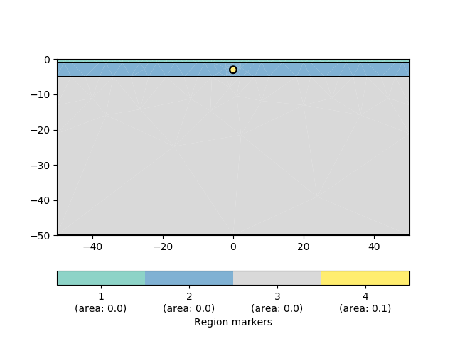
Create geometry definition for the modelling domain. worldMarker=True indicates the default boundary conditions for the ERT

world = mt.createWorld(start=[-50, 0], end=[50, -50], layers=[-1, -5],
                       worldMarker=True)

# Create some heterogeneous circular anomaly
block = mt.createCircle(pos=[0, -3.], radius=1, marker=4, boundaryMarker=10,
                        area=0.1)

# Merge geometry definition into a Piecewise Linear Complex (PLC)
geom = mt.mergePLC([world, block])

# Optional: show the geometry
pg.show(geom)

Create a Dipole Dipole (‘dd’) measuring scheme with 21 electrodes.

scheme = pb.createData(elecs=pg.utils.grange(start=-10, end=10, n=21),
                       schemeName='dd')

Put all electrodes (aka. sensors positions) into the PLC to enforce mesh refinement. Due to experience known, its convenient to add further refinement nodes in a distance of 10% of electrode spacing, to achieve sufficient numerical accuracy.

for pos in scheme.sensorPositions():
    geom.createNode(pos)
    geom.createNode(pos + pg.RVector3(0, -0.1))

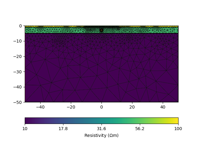
Create a mesh for the finite element modelling with appropriate mesh quality.

mesh = mt.createMesh(geom, quality=34)

# Create a map to set resistivity values in the appropriate regions
# [[regionNumber, resistivity], [regionNumber, resistivity], [...]
rhomap = [[1, 100.],
          [2, 50.],
          [3, 10.],
          [4, 100.]]

# Optional: take a look at the mesh
pg.show(mesh, data=rhomap, label='Resistivity $(\Omega$m)', showMesh=True)

Initialize the ERTManager (The class name is a subject to further change!)

ert = pb.ERTManager()

# Perform the modeling with the mesh and the measuring scheme itself
# and return a data container with apparent resistivity values,
# geometric factors and estimated data errors specified by the noise setting.
# The noise is also added to the data.
data = ert.simulate(mesh, res=rhomap, scheme=scheme, noiseLevel=1,
                    noiseAbs=1e-6)

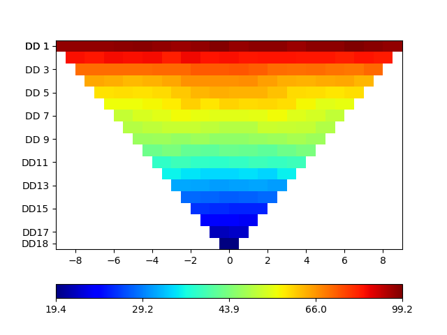
# Optional: you can filter all values and tokens in the data container.
print('Simulated rhoa', data('rhoa'), max(data('rhoa')))

# Its possible that there are some negative data values due to noise and
# huge geometric factors. So we need to remove them
data.markInvalid(data('rhoa') < 0)
print('Filtered rhoa', data('rhoa'), max(data('rhoa')))
data.removeInvalid()

# Optional: save the data for further use
data.save('simple.dat')

# Optional: take a look at the data
pb.show(data)

Out:

relativeError set to a value > 0.5 .. assuming this is a percentage Error level dividing them by 100
Data error estimate (min:max)  0.010000195282949438 : 0.011090363058703138
Simulated rhoa <class 'pygimli.core._pygimli_.RVector'> 171 [96.5888457117166,...,19.379920543633702] 99.22675013386537
Filtered rhoa <class 'pygimli.core._pygimli_.RVector'> 171 [96.5888457117166,...,19.379920543633702] 99.22675013386537

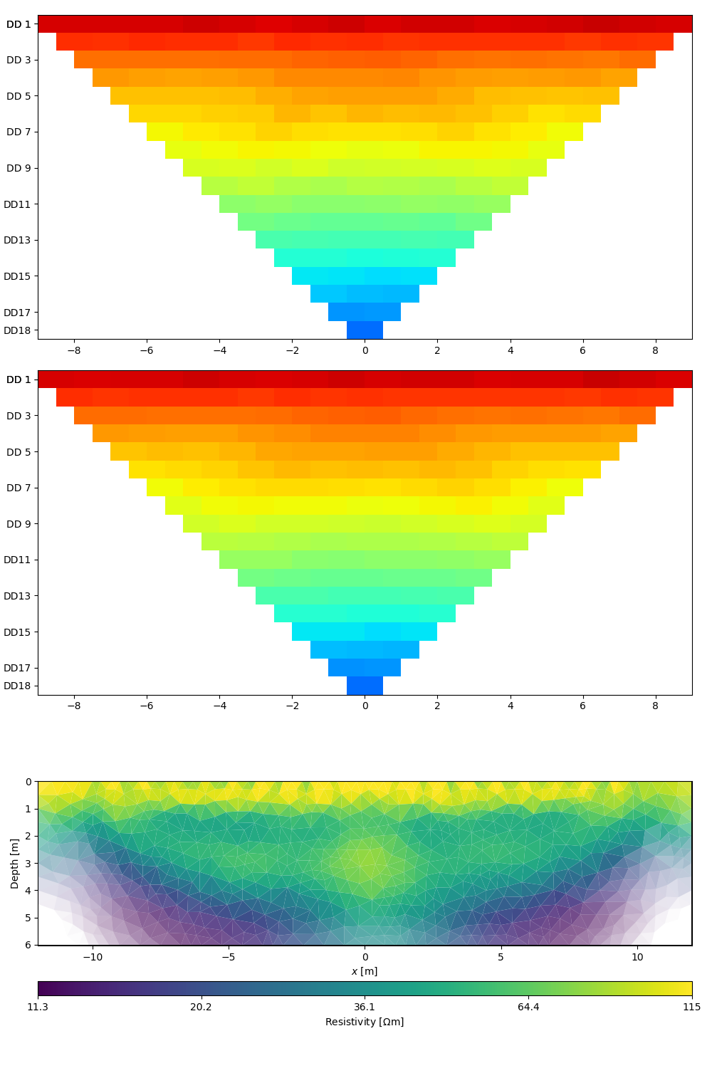
To avoid an inverse crime the inversion needs to be calculated on a different mesh that has no geometric signatures of the simulation mesh. Either let the inversion create a suitable mesh or provide a own.

# Run the ERTManager to invert the modeled data.
# The necessary inversion mesh is generated automatic.
model = ert.invert(data, paraDX=0.3, maxCellArea=0.2, lam=20)

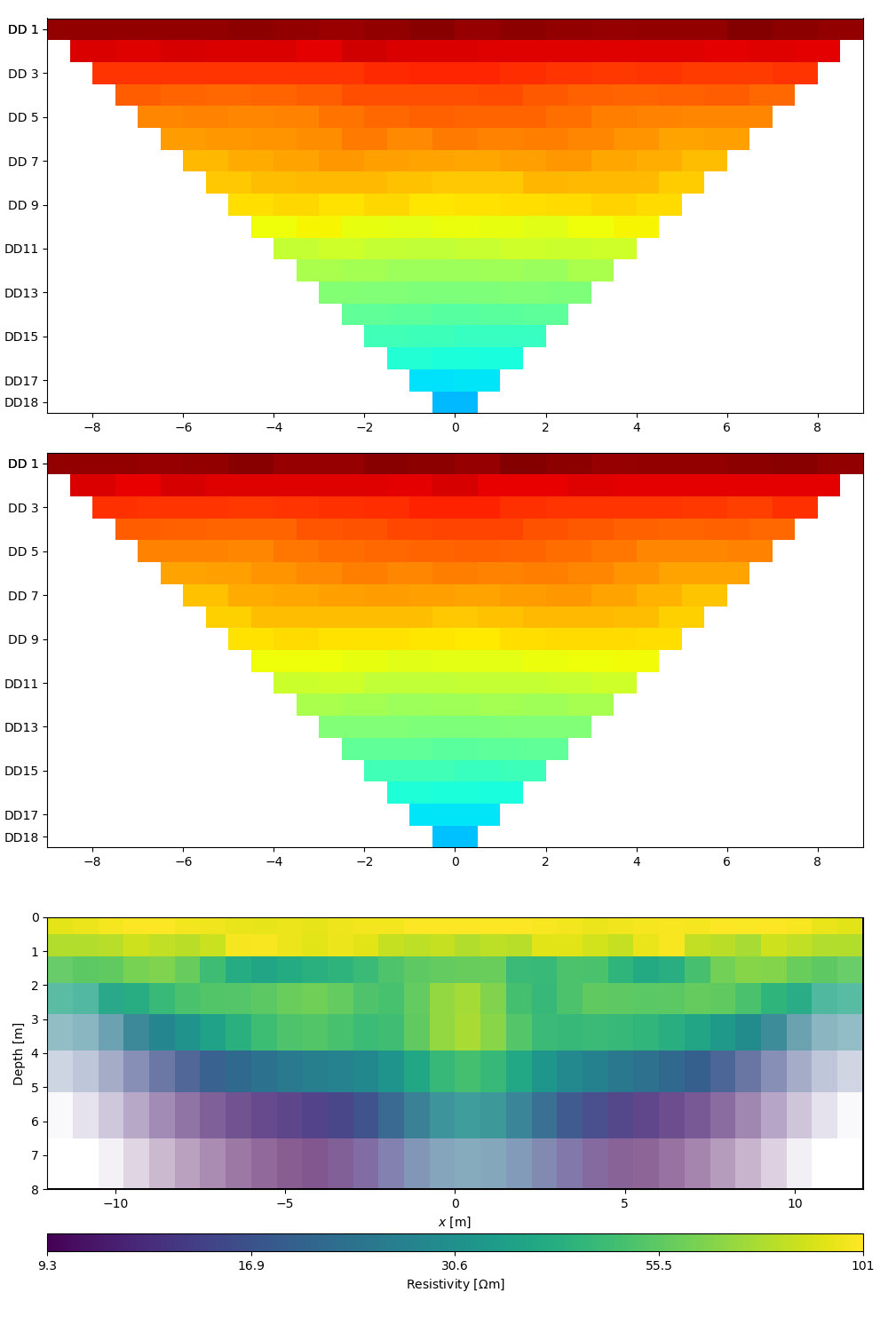
# Let the ERTManger show you the model and fitting results of the last
# successful run.
# Show data, model response, and model
ert.showResultAndFit()

Out:

creating mesh...
Mesh: Nodes: 1097 Cells: 2082 Boundaries: 3178
Mesh: Nodes: 1097 Cells: 2082 Boundaries: 3178

Optional: provide a custom mesh to the inversion

grid = pg.createGrid(x=pg.utils.grange(start=-12, end=12, n=33),
                     y=-pg.utils.grange(0.5, 8, n=8, log=True))

mesh = pg.meshtools.appendTriangleBoundary(grid, xbound=50, ybound=50)

model = ert.invert(data, mesh=mesh, lam=20)
ert.showResultAndFit()

chi2 = ert.inv.getChi2()

print(chi2)
# Stop the script here and wait until all figure are closed.
pg.wait()

Out:

Mesh: Nodes: 988 Cells: 1553 Boundaries: 2540
1.1657840287308814

Total running time of the script: ( 0 minutes 17.753 seconds)