DC2DInvRes - Constraints Menu
The dc resistivity inverse problem is ill-posed and non-unique.
We have to achieve uniqueness by regularization, e.g. by enforcing smooth models.
If we have additional information we can further restrict ambiguity resulting in more reliable models.
This may be the knownledge about the resistivity destribution or on the presence of layers, e.g. from other data or borehole investigations.
All this can interactively be done in the menu explained in the following.
See also the tutorial 4 for more examples.
Set as reference
If we know the subsurface in general (e.g. by geology or boreholes)
we expect the true resistivity distribution to be in the neighborhood of our concept.
By this option we change the reference model from the homogeneous half-space to the current model.
This may result from interpolation of pointwise information, from free hand modeling or from another inversion result loaded.
I suggest saving reference model so that several runs can be done easily.
Fix region
If the resistivity of a certain region is known, we can set it by free hand modeling.
If we furthermore want to exclude it from inversion we can fix it by using this option and drawing a rectangle thereafter.
The model cells are now marked with a white x each.
Typical cases are a well-known layer, a cavity or a water body of known resistivity.
Note that this feature can also be activated by typing "F" in the resistivity window.
Unfix region
By the way (drawing a rectangle) a region can loose its fix and the crosses will disappear.
Note that this feature can also be activated by typing "U" in the resistivity window.
Compound cells
If we know the resistivity to be constant in a certain region but we don't know the value
we can compound a number of cells in a way that their resistivities are clued together.
In the model cell this is depicted by white o's at the cells.
A typical case is a known clay layer or water table in depth.
Note that this feature can also be activated by typing "U" in the resistivity window.
Remove fix/compound
By this option all fixed or coumpounded region are removed.
This is automatically the case when loading data or an incompatible model from file.
Decoupling
Usually we impose smoothness constraints on the model resulting in blurred anomalies.
However, we can weight the individual model cell boundaries, e.g. by the blocky model option.
In presence of a known boundary the weight can be set to zero resulting in sharp gradients at this position.
Knowledge can come from borehole information, seismic or GPR surveys or observations at the surface.
Decouple x
A region is drought and all horizontal cell boundaries are decoupled in the inversion marked by a white "+" on the boundary.
Note that this feature can also be activated by typing "X" in the resistivity window.
Decouple z
A region is drought and all vertical cell boundaries are decoupled in the inversion also marked by a white "+".
The boundary might be a whole layer as the water table or piecewise as from cores or penetration tests.
Note that this feature can also be activated by typing "Z" in the resistivity window.
Borehole
One ore more boreholes on the profile can significantly improve our results.
By distincting different formations we allow the resistivity to jump in the neighborhood of the hole.
For automation I introduced a so-called bor-File (*.bor) that might be look as follows.
As for the data files, the "#" sign is used to form comments.
3 # three boreholes present
12.5 4 # 1st borehole position and number of layers
0 # humus layer (0 is a boundary anyway)
0.3 # sandy sediments
4.7 # water table
11 # clay
37 2 # 2nd borehole position and layers
5.6 # water table
11.5 # clay
55 # 3rd borehole
7 # water table, clay not found
Remove decoupling
All decouplings introduced before will be removed.
This is automatically the case when loading data or an incompatible model from file.
Underwater
When interpreting an underwater survey (with electrodes on ground) one wants to do two things:
-
The water resistivity shall be fixed to avoid artifacts.
-
At the ground a resistivity jump is expected and shall be enabled.
That's what the underwater mode is doing.
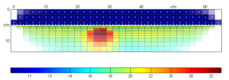
All cells above the electrodes (their depth may change as the seafloor does) are fixed.
A vertical decoupling is done, this may be the boundary below, above or both, depending on the position of the electrode inside the cell.
Don't forget to start with the water resistivity by typing it into the resistivity window and drawing a rectangle over the whole area.

Inversion result of a synthetic underwater study using a buried object.

